---
title: "Hypothesis tests"
author: "Steen Flammild Harsted & Søren O´Neill"
date: today
format:
html:
toc: true
toc-depth: 2
number-sections: true
number-depth: 2
code-fold: true
code-summary: "Show the code"
code-tools: true
execute:
eval: false
message: false
warning: false
---
<br><br>
# Presentation
You can download the course slides for this section <a href="./presentation_hypothesis_tests.html" download>here</a>
<div>
```{=html}
<iframe class="slide-deck" src="presentation_hypothesis_tests.html" width=90% ></iframe>
```
</div>
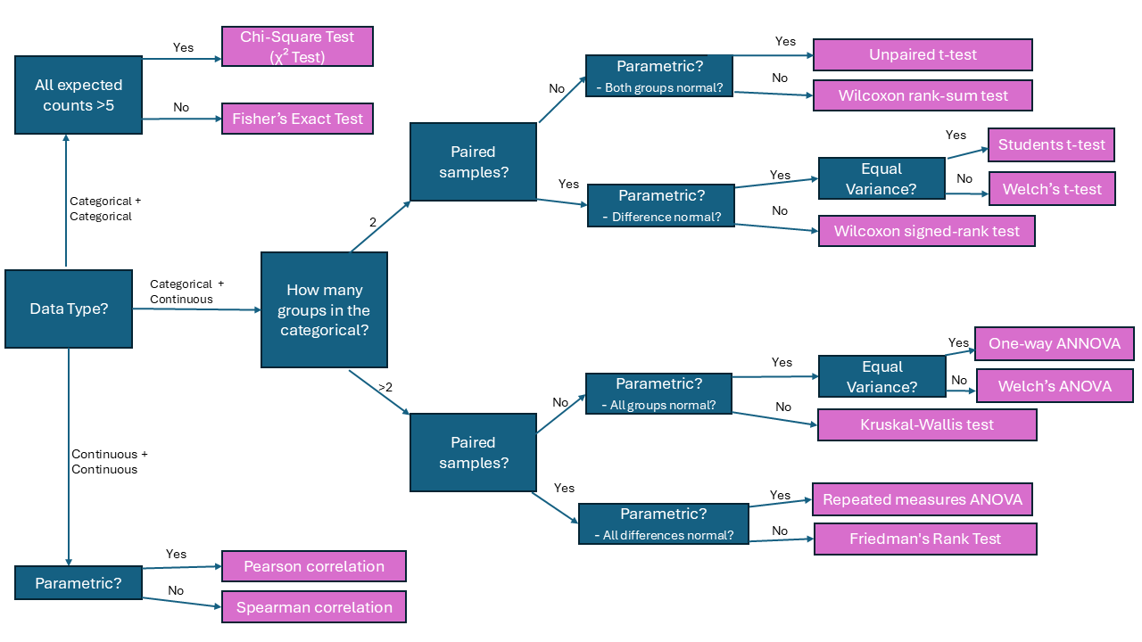
# Roadmap to your test
```{r}
#| column: page-inset-right
#| eval: true
#| echo: false
#| code-fold: false
#| lightbox:
#| group: r-graph
#| description: Roadmap to your test (r4phd.sdu.dk)
knitr::include_graphics(here::here("img", "hypo_tests.png"))
```
```{r setup}
#| include: false
#| echo: false
#| eval: true
library(tidyverse)
library(here)
library(gtsummary)
library(ggstatsplot)
library(rstatix)
library(statsExpressions)
#library(AER)
#library(easystats)
#library(GGally)
#library(gt)
#library(gtsummary)
#data("PhDPublications")
#library(palmerpenguins)
#source(here("scripts", "01_import.R"))
```
```{r}
#| eval: true
#| column: margin
#| echo: false
knitr::include_graphics(here::here("img", "sherif.png"))
```
## Getting Started {.unnumbered}
* Make sure that you are working in your course project
* Create a new quarto document and name it "hypothesis_tests.qmd"
* Insert a code chunk and load 2 important libraries
* Insert a new code chunk- Write `source(here("scripts", "01_import.R"))` in the chunk
* Write a short headline to each code chunk
* Change the YAML header to style your document output.
::: {.callout-tip collapse="true"}
### The YAML header can look like this
````{verbatim}
---
title: "TITLE"
subtitle: "SUBTITLE"
author: "ME"
date: today
format:
  html:
    toc: true
    toc-depth: 2
    embed-resources: true
    number-sections: true
    number-depth: 2
    code-fold: true
    code-summary: "Show the code"
    code-tools: true
execute:
  message: false
  warning: false
---
````
:::
<br><br>
<br>
#### Add the `gtsummary`, `ggstatsplot`, `statsExpressions` and `rstatix` packages to the code chunk where you have your library calls.
If you need to install any of the packages:
* use `install.packages(c("package_name", "package_name"))` to download the packages.
* This is done in the console and NOT in your script.
```{r}
#| eval: false
library(tidyverse)        # import, tidy, transform, visualize
library(here)             # filepath control
library(gtsummary)        # tables (with stats)
library(ggstatsplot)      # statistical plots
library(rstatix)          # statistical tests
library(statsExpressions) # statistical tests
```
<br><br>
## The `bugs_long` dataset
`bugs_long` provides information on the extent to which men and women want to kill arthropods that vary in disgustingness (low, high) and freighteningness (low, high) (four groups in total). Each participant rated their attitude towards all four kinds of anthropods. `bugs_long` is a subset of the data reported by [Ryan et al.(2013)](https://www.sciencedirect.com/science/article/abs/pii/S0747563213000277) .
`bugs_long` is included in the `ggstatsplot` package.
Note that this is a repeated measures design because the same participant gave four different ratings across four different conditions (LDLF, LDHF, HDLF, HDHF).
* `desire` - The desire to kill an arthropod was indicated on a scale from 0 to 10
* `gender` Male/Female
* `region`
* `condition`
- **LDLF**: low disgustingness and low freighteningness
- **LDHF**: low disgustingness and high freighteningness
- **HDLF**: high disgustingness and low freighteningness
- **HDHF**: high disgustingness and high freighteningness
```{r}
#| echo: false
#| eval: true
#| fig-cap: "Picture from Ryan et al. (2013) https://doi.org/10.1016/j.chb.2013.01.024"
knitr::include_graphics(here("img" , "bugs_conditions.jpg"))
```
<br><br>
### In `bugs_long`, is there a difference within the participants in their `desire` to kill bugs from the four different `conditions`?
* Should you use `ggwithinstats()` or `ggbetweenstats()` when comparing
* Is it reasonable to assume normality?
```{r}
bugs_long |> group_by(condition) |> shapiro_test(desire)

# qqplot
bugs_long |>
  ggplot(aes(sample = desire, group = condition)) +
  geom_qq_line(color = "red", linewidth = 1)+
  geom_qq()+
  facet_wrap(~condition)


# Density plot
bugs_long |>
  ggplot(aes(x = desire, fill = condition)) +
  geom_density(alpha = 0.2)
```
* Make the appropriate test
```{r}
#| code-summary: "`ggstatsplot`"
bugs_long |>
  ggwithinstats(x = condition,
                y = desire,
                type = "nonparametric")
```
```{r}
#| code-summary: "`rstatix`"
bugs_long |>

  # Friedman test only works with complete data
  # Some subjects have missing data in desire
  # We need to remove these
  drop_na(desire, condition, subject) |>
  add_count(subject) |>
  filter(n == 4) |>

  # Send the complete data
  friedman_test(desire ~ condition | subject)
```
```{r}
#| code-summary: "`statsExpressions`"
bugs_long |>
  oneway_anova(
    x = condition,
    y = desire,
    type = "nonparametric",
    paired = TRUE
  )
```
```{r}
#| code-summary: "`gtsummary`"
# This is not straightforward to do in gtsummary
# because you are looking at a repeated measures test (each subject has 4 rows)
#
# However, it can be done. See this link for how the author of the gtsummary package solves it
#
# https://stackoverflow.com/questions/75003882/how-to-do-repeated-measures-anova-and-friedman-test-in-gtsummary
```
* What is your interpretation?
* What is the consequence if you change the type of test?
<br><br>
### Is there a difference between men and women in the `desire` to kill bugs that are **LDHF** (low disgustingness and high freighteningness).
* Create a filtered data frame of bugs_long
```{r}
bugs_long_LDHF_only <- bugs_long |> filter(condition == "LDHF")
```
* Should you use `ggwithinstats()` or `ggbetweenstats()` for this test?
* Is it reasonable to assume normality?
```{r}
bugs_long_LDHF_only |>
  filter(!is.na(gender), !is.na(desire)) |>
  group_by(gender) |>
  shapiro_test(desire)

# qqplot
bugs_long_LDHF_only |>
  ggplot(aes(sample = desire, color = gender)) +
  geom_qq_line(color = "red", linewidth = 1) +
  geom_qq()+
  facet_wrap(~gender)


# Density plot
bugs_long_LDHF_only |>
  ggplot(aes(x = desire, fill = gender)) +
  geom_density(alpha = 0.2)
```
* Make the appropriate test
```{r}
#| code-summary: "ggstatsplot"
bugs_long_LDHF_only |>
  ggbetweenstats(x = gender,
                 y = desire,
                 type = "nonparametric")
```
```{r}
#| code-summary: "rstatix"
bugs_long_LDHF_only |>
  wilcox_test(desire ~ gender)
```
```{r}
#| code-summary: "statsExpressions"
bugs_long_LDHF_only |>
  two_sample_test(
    x = gender,
    y = desire,
    type = "nonparametric",
    paired = FALSE
  )
```
```{r}
#| code-summary: "gtsummary"
bugs_long_LDHF_only |>
  select(gender, desire) |>
  tbl_summary(by = "gender") |>
  add_p()
```
* What is your interpretation?
* What is the consequence if you change the type of test?
* Confused by all the different names in this example? Its not you. This test has many synonyms. Quote from [wikipedia](https://en.wikipedia.org/wiki/Mann%E2%80%93Whitney_U_test#:~:text=The%20Mann%E2%80%93Whitney%20U%20test%20%2F%20Wilcoxon%20rank%2Dsum%20test,to%20matched%20or%20dependent%20samples.): *"Mann–Whitney
U test (also called the Mann–Whitney–Wilcoxon (MWW/MWU), Wilcoxon rank-sum test, or Wilcoxon–Mann–Whitney test)..."*
<br><br>
### Is there a difference in the frequency of men and women between `North America` and the remaining regions?.
* First, lump `region` togehter to two levels (`fct_lump()`)
* Reduce the data to one row pr subject ID, and discuss why this is a good idea.
```{r}
bugs_long_region_lump <- bugs_long |>
  mutate(region = fct_lump(region, 1)) |>
  group_by(subject) |>
  slice(1) |>
  ungroup()
```
* Should you use `ggwithinstats()` or `ggbetweenstats()` or perhaps `ggbarstats()` for this test?
* Should you asses normality?
```{r}
# Both variables are factors (categorical/nominal). Normality has to do with continuous data
```
* Make the appropriate test
```{r}
#| code-summary: "ggstatsplot"
bugs_long_region_lump |>
  ggbarstats(x = gender,
             y = region)
```
```{r}
#| code-summary: "rstatix"
# rstatix is somewhat complicated here
# First we need to make table
# table is not pipe friendly

table(bugs_long_region_lump$region , bugs_long_region_lump$gender) |>

  # Then pass the table to the test
  chisq_test()
```
```{r}
#| code-summary: "statsExpressions"
bugs_long_region_lump |>
  contingency_table(gender, region)
```
```{r}
#| code-summary: "gtsummary"
# Notice that gtsummary is switching to Fishers exact test.
# Fishers exact test is actually the right tests to use if one of the groups has 5 or fewer observations
bugs_long_region_lump |>
  select(gender, region) |>
  tbl_summary(by = gender) |>
  add_p()

# If we absolutely want to run the chisquared test we do it like this
bugs_long_region_lump |>
  select(gender, region) |>
  tbl_summary(by = gender) |>
  add_p(test = list(all_categorical() ~ "chisq.test"))

# If you want to see a contigency table
# With row and column sum counts
bugs_long_region_lump |>
  drop_na() |> # Remove observations with missing values
  tbl_cross(gender, region) |>
  add_p()
```
* What is your interpretation?
<br><br>
## The `ToothGrowth` dataset
`ToothGrowth` gives information on tooth length in 60 guinea pigs. Each animal received one of three dose levels of vitamin C (0.5, 1, and 2 mg/day) by one of two delivery methods, orange juice or ascorbic acid (a form of vitamin C and coded as VC).
* `len` Tooth length
* `supp` Supplement type
- **VC** Vitamin C as ascorbic acid
- **OJ** Orange Juice
* `dose` Dose in milligrams/day (0.5, 1, or 2)
<br><br>
### Is there a difference in Tooth length based on the type of supplement?
* Should you use `ggwithinstats()` or `ggbetweenstats()` when comparing
* Is it reasonable to assume normality?
```{r}
ToothGrowth |> group_by(supp) |> shapiro_test(len)

# qqplot
ToothGrowth |>
  ggplot(aes(sample = len, color = supp)) +
  geom_qq()+
  geom_qq_line()

# Density plot
ToothGrowth |>
  ggplot(aes(x = len, fill = supp)) +
  geom_density(alpha = 0.2)
```
* Make the appropriate test
```{r}
#| code-summary: "ggstatsplot"
ToothGrowth |>
  ggbetweenstats(x = supp,
                 y = len,
                 type = "parametric")

# It is likely completely fine to run this as a "parametric" test, but you could consider type = "robust"
```
```{r}
#| code-summary: "rstatix"
ToothGrowth |>
  t_test(len ~ supp,
         paired = FALSE)

# We run this as a "parametric" test
```
```{r}
#| code-summary: "statsExpressions"
ToothGrowth |>
  two_sample_test(x = supp,
                  y = len,
                  paired = FALSE,
                  type = "parametric")

# It is likely completely fine to run this as a "parametric" test, but you could consider type = "robust".
```
```{r}
#| code-summary: "ggsummary"
ToothGrowth |>
  select(supp, len) |>
  tbl_summary(
    by = supp,
    statistic = list(all_continuous() ~ "{mean} ({sd})")) |>
  add_p(test = list(all_continuous() ~ "t.test"))
```
* What is your interpretation?
<br><br>
### Improve your home assignment
* Return to your home assignment and add some statistical tests if and where it makes sense
* Remember to change project (top right corner in Rstudio)
* Using the menu in the top right corner, you can switch between your course project and your home assignment